Steam quality calculation
1 Introduction
It can sometimes be interesting to calculate the vapourisation ratio of a mixture in a closed container, i.e. the mass fraction of vapour in the container. Such property is also known as the vapour quality [1].
Possible applications are related to fluid storage or selection of probe locations in containers whether they should be placed in the liquid or in the vapour.
So let’s first consider a closed container of volume \(V_T\) at a temperature \(T\) containing a total mole number of pure compound \(n_T\) (maybe another post could be dedicated to multicomponents mixtures). Schematically, at equilibrium the system can either be:
- fully liquid if \(V_T\) is lower than the pure compound volume in the container,
- fully gaseous if \(V_T\) is much much larger than the pure compound volume in the container,
- in gas-liquid equilibrium else.
In this post I will only focus on the gas-liquid and fully gaseous equilibrium states as we want to calculate the vapourisation ratio in the container at equilibrium.
2 System’s equilibrium modelling
2.1 Preliminary remark
An important thing to understand is that the whole container volume must be filled with material (liquid or vapour) at equilibrium. If not, this would imply that some portion of the container contains void thus has a pressure of zero (no pressure as there are no molecules). This is against the definition of a thermodynamic equilibrium which requires that a system at equilibrium is homogeneous in pressure (this can be false for systems with membranes and electrolytes). Therefore, there cannot be in the container a drop of liquid alone surrounded by void. If there is a drop of liquid then it is at equilibrium with its saturation vapour and the system’s pressure at temperature \(T\) is the so-called saturation pressure \(P^s\left(T\right)\).
2.2 Model’s equations
The mole balance on the species writes:
\[\begin{equation} n_T = n_L + n_G \tag{2.1} \end{equation}\]
with \(n_T\) the total mole amount of material in the container. \(n_L\) and \(n_G\) respectively are the mole numbers of the pure species in the liquid and the vapour phases.
Assuming that the gas phase follows the ideal gas law one can write:
\[\begin{equation} P^s v_G^s = RT \tag{2.2} \end{equation}\]
with \(v_G^s\) the saturated molar volume of the gas phase at equilibrium and \(R\) the ideal gas constant.
According to what was previously stated, the liquid and vapour phases occupy the total available volume:
\[\begin{equation} V_T = v_L^s \times n_L + v_G^s \times n_G \tag{2.3} \end{equation}\]
with \(v_L^s\) the saturated molar volume of the liquid phase at equilibrium.
It is also assumed that a relation between \(P^s\) and \(T\) such as the Antoine equation is known. Such correlation has the general form:
\[\begin{equation} P^s\left(T\right) = 10^{A-\frac{B}{C+T}} \tag{2.4} \end{equation}\]
with \(A\), \(B\) and \(C\) component specific parameters.
Moreover a relation between \(v_L^s\) and \(T\) such as the Rackett equation is assumed to be known. The DIPPR equation for \(v_L^s\) has the form:
\[\begin{equation} v_L^s\left(T\right) = M \times \left[\frac{A}{B^{1+\left(1-T/C\right)^D}}\right]^{-1} \tag{2.5} \end{equation}\]
with \(A\), \(B\), \(C\) and \(D\) component specific parameters. \(M\) is the species molecular weight.
The \(8\) variables of the model are: \(n_T\), \(n_L\), \(n_G\), \(P^s\), \(T\), \(V_T\), \(v_G^s\) and \(v_L^s\). The total number of equations is \(5\). Therefore one must specify \(3\) variables among the \(8\) to solve the problem. It is decided to specify \(n_T\), \(V_T\) and \(T\).
Remark 1: an equation of state such as the Peng-Robinson one would also allow the calculation of \(P^s\) and \(v_L^s\). For the sake of simplicity I prefer in this post to use correlations to explicitly estimate these properties with respect to temperature.
Remark 2: by imposing the initial material mass and the container total volume one imposes the molar density of the system at equilibrium \(\rho_T = n_T/V_T\). This quantity is therefore independent of the system final state (liquid, vapour or liquid-vapour), i.e. of the vapourisation ratio: it is an invariant of the system.
3 Resolution strategy
The system can be solved following these steps:
- select \(T\), \(V_T\) and \(n_T\) of the system
- calculate \(P^s\) and \(v_L^s\) using respectively Equations (2.4) and (2.5)
- calculate \(v_G^s\) using Equation (2.2)
- calculate \(n_L\) and \(n_G\) using Equations (2.1) and (2.3). Once combined, \(n_L\) and \(n_G\) expressions are:
\[\begin{equation} \left\{ \begin{aligned} n_L &= \frac{V_T - v_G^s \times n_T}{v_L^s - v_G^s} \\ n_G &= n_T - n_L \end{aligned} \right. \tag{3.1} \end{equation}\]
Above a certain temperature it is possible that the calculation leads to \(n_L\) values above \(n_T\) and negative \(n_G\) values. Such values have no physical meaning. In that case it should be considered that all liquid is vaporised and that \(n_G = n_T\) and \(n_L = 0\).
4 Application to water
Water is retained for example purpose as steam quality is an important topic for energetic cycles. The coefficients for \(P^s\) and \(v_L^s\) correlations of water are reported in Table 4.1.
| Property | Reference | A | B | C | D | Tmin (K) | Tmax (K) |
|---|---|---|---|---|---|---|---|
| \(P^s\) (mmHg) | [2] | 8.07131 | 1730.6300 | -39.724 | 274.15 | 372.15 | |
| \(v_L^s\) (kg/m3) | [3] | 0.14395 | 0.0112 | 649.727 | 0.05107 | 273.00 | 648.00 |
For the calculations it was assumed that 0.5 gram of water was trapped in a 1.5-liter container. Therefore density of the system is equal to \(0.33~kg.m^{-3}\).
Plot of the vapour fraction with respect to temperature is reported in Figure 4.1. For comparison purposes the quality calculated using Wagner’s equation of state [4] as programmed on the NIST website [5] is also represented on the same chart.
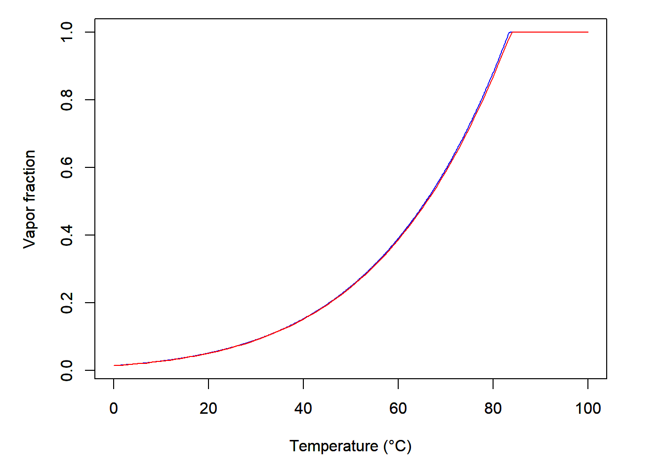
Figure 4.1: Vapor fraction with respect to temperature for 0.5 gram of water in a 1.5-liter container. Red line is calculated using the approach derived in this post. Bleu line is calculated using the NIST website tool.
One can see that the results are very similar: at low temperature almost no liquid is vaporised while liquid turns into vapour at high temperature. The vapour fraction increase is exponential as the saturation pressure \(P^s\) is also exponential with respect to temperature. Finally, the difference between the two curves might be explained by different values of \(P^s\) and \(v_L^s\) calculated depending on if the correlations or the equation of state is used.
In conclusion, the approach suggested in this post seems to be validated as the results from both approaches are very close (and I’m not gonna criticize NIST’s results on water, I’m not a fool…).