Penduluuuuuuuum
1 Introduction
The purpose of this post is to derive and solve the equation of motion of a pendulum attached to a moving board. The board can only slide following an horizontal line. The board can move according to the motion law \(b\left(t\right)\). The \(b\) expression has no restriction. From its equation, it is possible to know the velocity and acceleration of the board by calculating \(\dot{b}\) and \(\ddot{b}\).
The second law of Newton will be applied to the mass at the end of the pendulum which is subject to gravitational force (vertical force) and the string force (pointing from the mass to its attachment point), respectively noted \(m\overrightarrow{g}\) and \(\overrightarrow{F}\) in figure 2.1.
2 Referential selection
Two different referential, as represented in figure 2.1, can be relevant for the analysis of the system:
a static referential in which the board is having an horizontal movement only and relevant to describe the board motion. The referential is built upon the two orthogonal unit vectors \(\overrightarrow{e}_x\) and \(\overrightarrow{e}_y\). Yet, in this referential, the string reaction has two contributions \(F_x\) and \(F_y\) which are unknown. Therefore, when the second law of Newton is applied, a system of two equations (force balance along the \(\overrightarrow{e}_x\) and \(\overrightarrow{e}_y\) directions) and three unknowns (\(\theta\), \(F_x\) and \(F_y\)) will be derived. Therefore, the problem will be intractable (note from the future: the last statement is incorrect as the derivation is much easier to perform by working mainly, but not exclusively, in this referential. The trick is only to go the the moving refrential at a specific moment of the derivation as explained later is this post).
a dynamic referential attached to the mass and relevant to describe the pendulum motion (called pendulum referential). The referential is built upon the two orthogonal unit vectors \(\overrightarrow{e}_{\theta}\) and \(\overrightarrow{e}_r\). In this referential, the string reaction has one contribution \(F_{\theta}\) which is unknown. Therefore, When the second law of Newton is applied, the force balance along the \(\overrightarrow{e}_r\) direction will only have \(\theta\) as unknown. Therefore, the problem will be tractable (note from the future: yes it can be solved… but it is a pain).
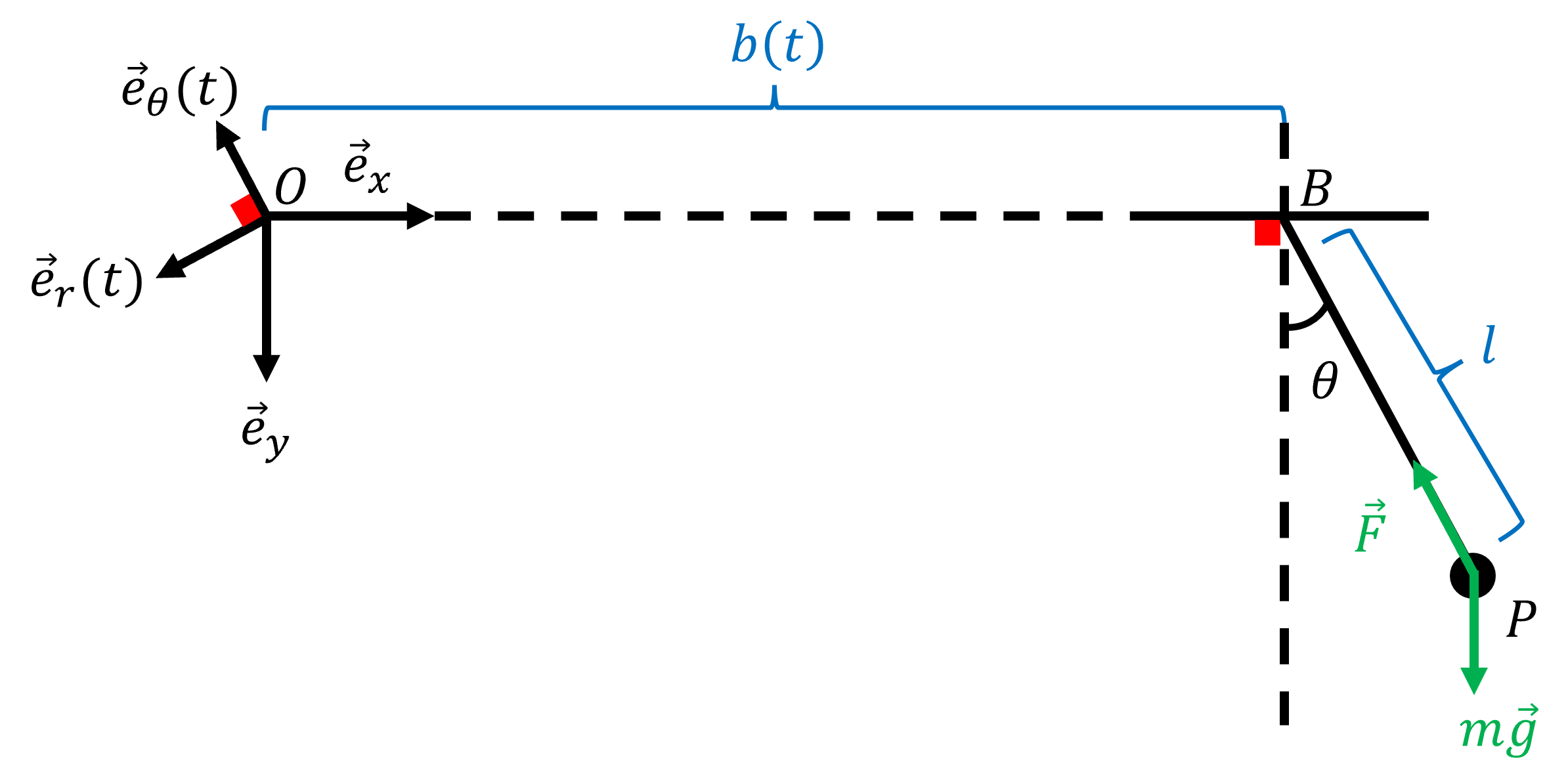
Figure 2.1: Two possible referentials for the pendulum analysis
In figure 2.1, the pendulum length is noted \(l\) and is a constant (no elastic behavior) and \(\theta\) is the pendulum angle with respect to the vertical axis.
Whatever is the selected referential, the first work to do is to derive an expression of \(\overrightarrow{OP}\) that will be derived twice with respect to time when Newton’s second law is applied.
3 Derivation of the motion equation using the rotating referential
TL;DR: this derivation is based on geometric considerations and definitely too long. Although correct, another path is proposed in the next section. However, this section has the benefit to show an alternative way to obtain the expected result.
The hard part of this problem is therefore to express vector \(\overrightarrow{OP}\) in the pendulum referential. As illustrated in figure 3.1, some additional points must be defined to perform further calculations:
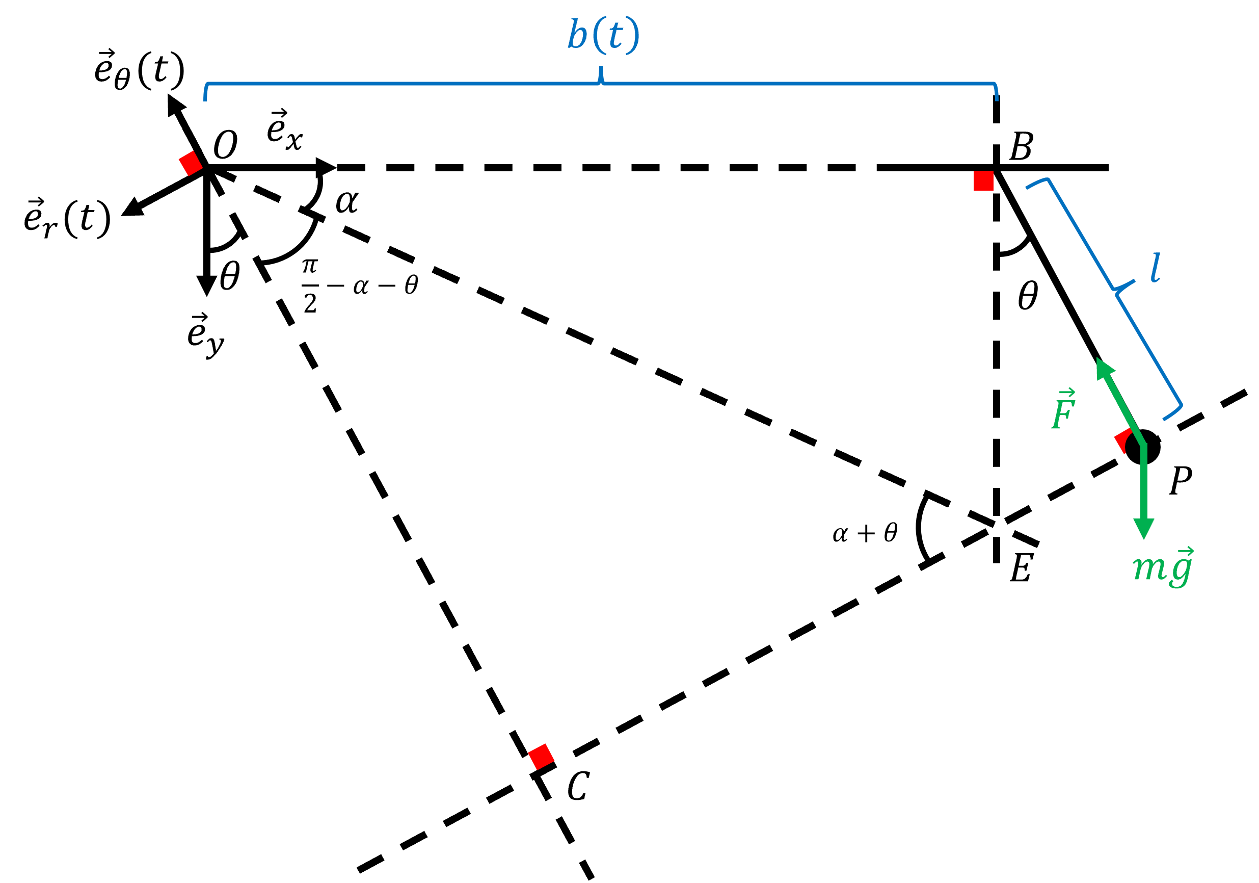
Figure 3.1: Definition of some points and angles for this first derivation
- \(C\) is the intersection between the line collinear to \(\overrightarrow{e}_{\theta}\) and the line perpendicular to segment \(BP\) and intersecting \(P\). Therefore, \(\angle{OCP}=90°\). Moreover, because \(OC\) and \(BP\) are both perpendicular to \(CP\) they are parallel. Therefore, \(\angle{COe_y}=\theta\).
- \(E\) is the intersection between \(CP\) and the line perpendicular to \(OB\) and crossing \(B\). We additionally define \(\alpha = \angle{BOE}\).
- Because \(\angle{e_xOe_y=90°}\), \(\angle{COE}=\pi/2-\alpha-\theta\).
- Because the sum of triangle’s OCE angles has to be 180°, \(\angle{CEO=\alpha+\theta}\)
From figure 3.1, one can see that \(\overrightarrow{OP}\) can be expressed as:
\[\begin{equation} \overrightarrow{OP} = OC \times \left(-\overrightarrow{e}_{\theta}\right) + CP \times \left(-\overrightarrow{e}_{r}\right) \tag{3.1} \end{equation}\]
Therefore, the objective is to derive \(OC\) and \(CP\) expressions involving \(\theta\), \(b\) and \(l\).
3.1 Derivation of \(OC\) expression
One can see in triangle \(OCE\) that:
\[\begin{equation} \sin{\left(\alpha+\theta\right)} = \frac{OC}{OE} \Leftrightarrow OC = OE \times \sin{\left(\alpha+\theta\right)} \tag{3.2} \end{equation}\]
Moreover, in triangle \(OBE\):
\[\begin{equation} \cos{\alpha} = \frac{b}{OE} \Leftrightarrow OE = \frac{b}{\cos{\alpha}} \tag{3.3} \end{equation}\]
Combining (3.2) and (3.3), one finds:
\[\begin{equation} OC = b\times \frac{\sin{\left(\alpha+\theta\right)}}{\cos{\alpha}} \tag{3.4} \end{equation}\]
We want to get ride of the \(\alpha\) terms to only have an expression using \(\theta\) (otherwise we will have too many unknowns for the set of equations derived from Newton’s second law). One can remember that \(\sin{\left(\alpha+\theta\right)} = sin{\alpha} \cos{\theta} + sin{\theta} \cos{\alpha}\). Therefore, (3.4) becomes:
\[\begin{equation} OC = b\times \frac{sin{\alpha} \cos{\theta} + sin{\theta} \cos{\alpha}}{\cos{\alpha}} = b\times \left(tan{\alpha} \cos{\theta} + sin{\theta}\right) \tag{3.5} \end{equation}\]
Now only \(\tan{\alpha}\) remains to be removed. By looking at triangle \(OBE\), one sees that:
\[\begin{equation} \tan{\alpha} = \frac{BE}{b} \tag{3.6} \end{equation}\]
And by looking at triangle \(BEP\), one finds that:
\[\begin{equation} cos{\theta} = \frac{l}{BE} \tag{3.7} \end{equation}\]
Therefore, combining equations (3.6) and (3.7), one finds that:
\[\begin{equation} \tan{\alpha} = \frac{l}{b \cos{\theta}} \tag{3.8} \end{equation}\]
Finally, the \(OC\) expression from (3.5) becomes:
\[\begin{equation} OC = b \times \left(\frac{l}{b\cos{\theta}} \times \cos{\theta}+ \sin{\theta}\right) = l+b \sin{\theta} \tag{3.9} \end{equation}\]
3.2 Derivation of \(CP\) expression
In triangle \(OCE\), one can derive:
\[\begin{equation} \cos{\alpha+\theta} = \frac{CE}{OE} = \frac{CE \cos{\alpha}}{b} \Leftrightarrow CE = b \times \frac{\cos{\alpha+\theta}}{\cos{\alpha}} \tag{3.10} \end{equation}\]
One can remember that \(\cos{\left(\alpha+\theta\right)} = cos{\alpha} \cos{\theta} - sin{\theta} \sin{\alpha}\). Therefore:
\[\begin{equation} CE = b \times \frac{cos{\alpha} \cos{\theta} - sin{\theta} \sin{\alpha}}{\cos{\alpha}} = b \times \left(\cos{\theta} - \sin{\theta} \tan{\alpha}\right) \tag{3.11} \end{equation}\]
Injecting equation (3.8) in (3.11):
\[\begin{equation} CE = b \times \left(\cos{\theta} - \sin{\theta} \frac{l}{b \cos{\theta}}\right) = b \cos{\theta} - l \tan{\theta} \tag{3.12} \end{equation}\]
Because \(CP = CE + EP\) and that in triangle \(BEP\) one sees that \(\tan{\theta} = EP/l\) one finally finds:
\[\begin{equation} CP = b \cos{\theta} - l \tan{\theta} + l \tan{\theta} = b \cos{\theta} \tag{3.13} \end{equation}\]
From equations (3.9) and (3.13), one has:
\[\begin{equation} \overrightarrow{OP} = \left(l+b \sin{\theta}\right) \times \left(-\overrightarrow{e}_{\theta}\right) + b \cos{\theta} \times \left(-\overrightarrow{e}_{r}\right) \tag{3.14} \end{equation}\]
3.3 Expression of \(\overrightarrow{OP}\) derivatives with respect to time
The unit vectors \(\overrightarrow{e}_{r}\) and \(\overrightarrow{e}_{\theta}\) will move with time. Indeed, the direction of these vectors is directly related to the value of \(\theta\) which varies with time. Therefore, these vectors must be derived when the derivatives of \(\overrightarrow{OP}\) will be calculated. To find these derivatives, the simplest is to express \(\overrightarrow{e}_{r}\) and \(\overrightarrow{e}_{\theta}\) in the other referential defined by vectors \(\overrightarrow{e}_{x}\) and \(\overrightarrow{e}_{y}\) which do not move with time. From figure 3.1, one can see that:
\[\begin{equation} \overrightarrow{e}_{\theta} = -\sin{\theta} \times \overrightarrow{e}_{x} - \cos{\theta} \times \overrightarrow{e}_{y} \tag{3.15} \end{equation}\]
and
\[\begin{equation} \overrightarrow{e}_{r} = -\cos{\theta} \times \overrightarrow{e}_{x} + \sin{\theta} \times \overrightarrow{e}_{y} \tag{3.16} \end{equation}\]
Therefore, \(d\overrightarrow{e}_{\theta}/dt\) and \(d\overrightarrow{e}_{r}/dt\) can be calculated:
\[\begin{equation} \frac{d\overrightarrow{e}_{\theta}}{dt} = -\dot{\theta}\cos{\theta} \times \overrightarrow{e}_{x} + \dot{\theta}\sin{\theta} \times \overrightarrow{e}_{y} = \dot{\theta} \times \overrightarrow{e}_{r} \tag{3.17} \end{equation}\]
and
\[\begin{equation} \frac{d\overrightarrow{e}_{r}}{dt} = \dot{\theta}\sin{\theta} \times \overrightarrow{e}_{x} + \dot{\theta}\cos{\theta} \times \overrightarrow{e}_{y} = - \dot{\theta} \times \overrightarrow{e}_{\theta} \tag{3.18} \end{equation}\]
Now, one can calculate the first derivative of \(\overrightarrow{OP}\) derivatives with respect to time:
\[\begin{equation} \frac{d\overrightarrow{OP}}{dt} = \left(\dot{b} \sin{\theta} + b\dot{\theta}\cos{\theta}\right) \times \left(-\overrightarrow{e}_{\theta}\right) + \left(l+b\sin{\theta}\right)\times\left(-\dot{\theta} \times \overrightarrow{e}_{r}\right) + \left(\dot{b}\cos{\theta} - b\dot{\theta}\sin{\theta}\right) \times \left(-\overrightarrow{e}_{r}\right) + b \cos{\theta} \times \dot{\theta} \times \overrightarrow{e}_{\theta} \tag{3.19} \end{equation}\]
Some terms cancel. Once the simplifications are done, one obtains:
\[\begin{equation} \frac{d\overrightarrow{OP}}{dt} = -\dot{b} \sin{\theta} \times \overrightarrow{e}_{\theta}+ \left(-l\dot{\theta} - \dot{b}\cos{\theta}\right) \times \overrightarrow{e}_{r} \tag{3.20} \end{equation}\]
The second derivative of \(\overrightarrow{OP}\) can be calculated:
\[\begin{equation} \frac{d^2\overrightarrow{OP}}{dt^2} = \left(-\ddot{b}\sin{\theta}-\dot{b}\dot{\theta}\cos{\theta}\right) \times \overrightarrow{e}_{\theta} - \dot{b} \dot{\theta} \sin{\theta} \times\overrightarrow{e}_{r} + \left(-l\ddot{\theta} - \ddot{b}\cos{\theta} + \dot{b}\dot{\theta} \sin{\theta}\right) \times\overrightarrow{e}_{r} - \left(-l\dot{\theta} - \dot{b}\cos{\theta}\right) \dot{\theta} \times \overrightarrow{e}_{\theta} \tag{3.21} \end{equation}\]
Once the simplifications are done, one obtains:
\[\begin{equation} \frac{d^2\overrightarrow{OP}}{dt^2} = \left(-\ddot{b}\sin{\theta} + l \dot{\theta}^2\right) \times \overrightarrow{e}_{\theta} + \left(-l\ddot{\theta} - \ddot{b}\cos{\theta}\right) \times\overrightarrow{e}_{r} \tag{3.22} \end{equation}\]
4 Derivation of the motion equation using the static referential
This derivation came to my mind after seeing the simple result obtained from the first derivation. It is so simple that I believe the path I followed was not the simplest one. Indeed, I came to the conclusion that the derivation can be done mostly in the static referential and just at the end switch to the rotating referential using the relations between vectors \(\overrightarrow{e}_{r}\), \(\overrightarrow{e}_{\theta}\), \(\overrightarrow{e}_{x}\) and \(\overrightarrow{e}_{y}\).
The \(\overrightarrow{OP}\) array writes:
\[\begin{equation} \overrightarrow{OP} = \left(b+l \sin{\theta}\right)\times \overrightarrow{e}_{x} + l \cos\theta\times \overrightarrow{e}_{y} \tag{4.1} \end{equation}\]
The derivative of (4.1) is straight forward:
\[\begin{equation} \frac{d\overrightarrow{OP}}{dt} = \left(\dot{b}+l \dot{\theta} \cos{\theta}\right)\times \overrightarrow{e}_{x} - l \dot{\theta}\sin\theta\times \overrightarrow{e}_{y} \tag{4.2} \end{equation}\]
The derivative of (4.2) is also straight forward:
\[\begin{equation} \frac{d^2\overrightarrow{OP}}{dt^2} = \left(\ddot{b}+l \ddot{\theta} \cos{\theta} - l\dot{\theta}^2 \sin{\theta}\right)\times \overrightarrow{e}_{x} - \left(l\ddot{\theta}\sin\theta + l\dot{\theta}^2 \cos{\theta}\right)\times \overrightarrow{e}_{y} \tag{4.3} \end{equation}\]
\(\overrightarrow{e}_{y}\) can be expressed as:
\[\begin{equation} \overrightarrow{e}_{y} = -\cos{\theta} \times \overrightarrow{e}_{\theta} + \sin{\theta} \times \overrightarrow{e}_{r} \tag{4.4} \end{equation}\]
Similar equation for \(\overrightarrow{e}_{x}\) can be derived:
\[\begin{equation} \overrightarrow{e}_{x} = -\sin{\theta} \times \overrightarrow{e}_{\theta} - \cos{\theta} \times \overrightarrow{e}_{r} \tag{4.5} \end{equation}\]
Therefore, equation (4.3) becomes:
\[\begin{equation} \frac{d^2\overrightarrow{OP}}{dt^2} = \left(\ddot{b}+l \ddot{\theta} \cos{\theta} - l\dot{\theta}^2 \sin{\theta}\right)\times \left(-\sin{\theta} \overrightarrow{e}_{\theta} - \cos{\theta} \overrightarrow{e}_{r}\right) - \left(l\ddot{\theta}\sin\theta + l\dot{\theta}^2 \cos{\theta}\right)\times \left(-\cos{\theta} \overrightarrow{e}_{\theta} + \sin{\theta} \overrightarrow{e}_{r}\right) \tag{4.6} \end{equation}\]
After development and simplification, one finds:
\[\begin{equation} \frac{d^2\overrightarrow{OP}}{dt^2} = \left(-\ddot{b}\sin{\theta} + l \dot{\theta}^2\right) \times \overrightarrow{e}_{\theta} + \left(-l\ddot{\theta} - \ddot{b}\cos{\theta}\right) \times\overrightarrow{e}_{r} \tag{4.7} \end{equation}\]
which is the same equation as (3.22). One notices that this path to estimate \(d^2\overrightarrow{OP}/dt^2\) is indeed faster🥳.
5 Application of Newton’s second law
Newton’s second law applied to the pendulum mass writes:
\[\begin{equation} m \frac{d^2\overrightarrow{OP}}{dt^2} = m \overrightarrow{g} + \overrightarrow{F} = mg \times \overrightarrow{e}_y + F \times \overrightarrow{e}_{\theta} \tag{5.1} \end{equation}\]
Multiplying equation (3.15) by \(-\cos{\theta}\) and (3.16) by \(\sin{\theta}\) and summing the two equations, one obtains (4.4) again, i.e.,:
\[\begin{equation} \overrightarrow{e}_y = -\cos{\theta} \times \overrightarrow{e}_{\theta} + \sin{\theta} \times \overrightarrow{e}_{r} \tag{5.2} \end{equation}\]
Therefore, equation (5.1) rewrites:
\[\begin{equation} m \frac{d^2\overrightarrow{OP}}{dt^2} = mg \times \left(-\cos{\theta} \times \overrightarrow{e}_{\theta} + \sin{\theta} \times \overrightarrow{e}_{r}\right) + F \times \overrightarrow{e}_{\theta} \tag{5.3} \end{equation}\]
Finally, the set of equations describing pendulum motion is:
\[\begin{equation} -\ddot{b}\sin{\theta} + l \dot{\theta}^2 = -g \cos{\theta} + F/m \tag{5.4} \end{equation}\]
\[\begin{equation} -l\ddot{\theta} - \ddot{b}\cos{\theta} = g \sin{\theta} \tag{5.5} \end{equation}\]
The equation not involving the string reaction \(F\) can be rewritten:
\[\begin{equation} \ddot{\theta} + \frac{g}{l} \sin{\theta} + \frac{\ddot{b}}{l}\cos{\theta} = 0 \tag{5.6} \end{equation}\]
which reduces to the classical static pendulum equation if the board is static (i.e. \(b\) is constant and \(\ddot{b}=0\)).
6 Analytical solutions
6.1 Small oscillations
In the case of small oscillations, \(\theta\) will remain close to zero and under this assumption, \(\sin{\theta} \approx \theta\) and \(\cos{\theta} \approx 1\). Therefore, equation (5.6) becomes:
\[\begin{equation} \ddot{\theta} + \frac{g}{l} \theta + \frac{\ddot{b}}{l} = 0 \tag{6.1} \end{equation}\]
According to Wolfram Alpha, the solution of this differential equation is:
\[\begin{equation} \theta\left(t\right) = \underbrace{C_1 \sin{\left(\sqrt{\frac{g}{l}}t\right)} + C_2 \cos{\left(\sqrt{\frac{g}{l}}t\right)}}_{\text{static pendulum classical solution}} + \sin{\left(\sqrt{\frac{g}{l}}t\right)} \int_1^t{-\frac{\ddot{b}\left(\xi\right) \cos{\left(\frac{g}{l}\xi\right)}}{\sqrt{gl}} d\xi} + \cos{\left(\sqrt{\frac{g}{l}}t\right)} \int_1^t{\frac{\ddot{b}\left(\xi\right) \sin{\left(\frac{g}{l}\xi\right)}}{\sqrt{gl}} d\xi} \tag{6.2} \end{equation}\]
It is likely that the integrals might not have an analytical solution depending on the \(\ddot{b}\) expression used. Therefore, numerical resolution will have to be performed, even for the small oscillations problem.
6.2 Constant angle
If one wants to know what the \(\ddot{b}\) expression must be so that the pendulum angle does not move, one can solve equation (5.6) with \(\theta=\theta_0\) with \(\theta_0\) the pendulum angle at the initial time. Therefore:
\[\begin{equation} \frac{g}{l} \sin{\theta_0} + \frac{\ddot{b}}{l}\cos{\theta_0} = 0 \tag{6.3} \end{equation}\]
Therefore, \(\ddot{b}\) is:
\[\begin{equation} \ddot{b} = -g\tan{\theta_0} \tag{6.4} \end{equation}\]
The solution to this differential equation, assuming an initially still board and centered in \(x=0\) is:
\[\begin{equation} b\left(t\right) = -\frac{1}{2}gt^2\tan{\theta_0} \tag{6.4} \end{equation}\]
It is interesting to notice that this equation diverges when \(\theta_0=\pi/2\) (i.e., it is not possible to maintain a constant angle of 90° for the pendulum).
7 Simulation
The differential equation solving procedure was coded in Python using scipy for the integration procedure and animation library to achieve a dynamic plotting.
7.1 Python code
Only few parameters should be changed for your personal use:
HISTORY_LENto adjust simulation timeboard_function(t)to define your own board movement equationLENGTHfor the rope length
import numpy as np
from scipy.integrate import odeint
import matplotlib.pyplot as plt
import matplotlib.animation as animation
from collections import deque

# Constants
HISTORY_LEN = 500  # Number of trajectory points to display
TEND = 20  # Simulation time in s
DT = 0.02  # Calculation interval in s
NSTEP = int(TEND / DT)


def board_function(t):
    return np.sin(t)


def second_derivative_board_function(t):
    eps = DT / 100
    return (board_function(t + eps) - 2 * board_function(t) + board_function(t - eps)) / eps ** 2


def pendulum_ode(y, t, gravity, length):
    theta, theta_dot = y
    dydt = [theta_dot, -gravity / length * np.sin(theta) - second_derivative_board_function(t) / length * np.cos(theta)]
    return dydt


def animate(time_step):
    thisx = [xb[time_step], xp[time_step]]
    thisy = [yb[time_step], yp[time_step]]

    if time_step == 0:
        history_x.clear()
        history_y.clear()

    history_x.appendleft(thisx[1])
    history_y.appendleft(thisy[1])

    line.set_data(thisx, thisy)
    trace.set_data(history_x, history_y)
    time_text.set_text(time_template % (time_step * DT))
    return line, trace, time_text


if __name__ == '__main__':
    t = np.linspace(0, TEND, NSTEP)
    y0 = [np.pi/4, 0]
    GRAVITY = 9.81  # m.s-2
    LENGTH = 1  # m

    sol = odeint(pendulum_ode, y0, t, args=(GRAVITY, LENGTH))

    # Calculate coordinates
    xb = [board_function(ti) for ti in t]
    yb = [0] * len(t)
    xp = [board_function(ti) + LENGTH * np.sin(sol[i, 0]) for i, ti in enumerate(t)]
    yp = [-LENGTH * np.cos(sol[i, 0]) for i in range(len(sol[:, 0]))]

    # xp = xp / np.max(np.abs(xb))
    # xb = xb / np.max(np.abs(xb))

    fig = plt.figure(figsize=(10, 10))

    # Calculate bmin and bmax
    bmin = min(xb)
    bmax = max(xb)

    ax = fig.add_subplot(autoscale_on=False, xlim=(bmin-LENGTH, bmax+LENGTH), ylim=(-LENGTH, LENGTH))
    ax.set_aspect('equal')
    ax.grid()

    line, = ax.plot([], [], 'o-', lw=2)
    trace, = ax.plot([], [], '.-', lw=1, ms=2)
    time_template = 'time = %.1fs'
    time_text = ax.text(0.05, 0.9, '', transform=ax.transAxes)
    history_x, history_y = deque(maxlen=HISTORY_LEN), deque(maxlen=HISTORY_LEN)

    ani = animation.FuncAnimation(fig, animate, len(sol[:, 0]), interval=DT * 500, blit=True)
    plt.show()
7.2 Results
The pendulum length was assumed to be 1 meter for all simulations but the last one. Indeed, in order to have a plot of acceptable size, I needed to assume a pendulum of 1 km. However, the result should not be impacted by this change.
7.2.1 Still board
- Initial pendulum angle is 45° (cf. figure 7.1): an oscillation of the pendulum is obtained. So far, no surprise, it was just to check that the calculation was consistent for this simple case.
Figure 7.1: Still board with initial pendulum angle of 45°
- Initial pendulum angle is 180° (cf. figure 7.2). The pendulum is stable for the 20 seconds of simulation. I was not sure that it would be the case as numerical errors do exist and could have increased leading to reaching a value of the pendulum angle slightly different from 180°, yet sufficient, to initiate a swing. This setup is known as the inverse pendulum.
Figure 7.2: Still board with initial pendulum angle of 180°
7.2.2 Moving board
- Sinusoidal displacement of the board (\(b\left(t\right) = \sin\left(t\right)\)) with initial pendulum angle of 45° (cf. figure 7.3). Here starts the fun. It seems that for this condition, the pendulum describes a “bretzel” shape. Not enough to win a Nobel prize, yet fun to see 😁.
Figure 7.3: Sinusoidal board movement with initial pendulum angle of 45°
- Sinusoidal displacement of the board (\(b\left(t\right) = \sin\left(t\right)\)) with initial pendulum angle of 90° (cf. figure 7.4). It is interesting to observe that the pattern drawn by the pendulum is different when changing its initial angle. Again, nothing amazing but I have the intuition that it should be possible to draw some nice pictures with a nice set of conditions (initial pendulum angle, board displacement over time).
Figure 7.4: Sinusoidal board movement with initial pendulum angle of 90°
- Sinusoidal displacement of the board (\(b\left(t\right) = \sin\left(t\right) + \sin\left(t/3\right)\)) with initial pendulum angle of 45° (cf. figure 7.5). With this one it is interesting to see that the combination of two sinus curves to express the board displacement can already lead to complex patters for the pendulum movement. I believe that the coefficients of the sinus terms from the board displacement equation can be estimated performing the harmonic analysis of the pendulum position over time. Maybe for a next time.
Figure 7.5: Double sinusoidal board movement
- Constant angle solution (cf. figure 7.6). The initial pendulum angle is set to 45°. This one was just to check that equation (6.4) was correct. And yes it is 😎.
Figure 7.6: Board displacement to maintain pendulum angle
8 Conclusions and possible next steps
This post was the occasion to perform some work around the pendulum how it behaves when attached to a moving board. It appeared that the derivation can either be very complicated only following my first intuition while much simpler when taking some minutes to think about why the motion equation, at the end, is so simple. The fun part of this post remains the simulation of some scenarios with still and moving board. It is very nice not to limit ourselves to some analytical solutions but to be able to numerically solve the equation of motion for all possible conditions and not only small angle oscillations.
It is clear that this system is an open door for other discussions such as:
- PID regulation in the case of the inverse pendulum when small perturbations would lead to pendulum to fall: how should the board react?
- Harmonic analysis of the pendulum motion when the board move is a combination of sinusoidal curves
- Extension to the double pendulum case with the moving board: can the chaotic behavior of the double pendulum be reduced with the moving board? Or is it worse?
- Extension to the infinite pendulum (infinite number of pendulum attached together in series) to represent a rope
- Accounting for air friction to avoid perpetual motion
- Replacement of the solid rope by a spring: why not after all 🤪