Gaussian curve parameterization for chromatography
1 Introduction
In chromatography, one can represent the output of a small sample injection over time as a gaussian curve. To do so, one must parameterize the gaussian curve in order to reproduce: the retention time, the peak height and the peak width at half-height.
According to Wikipedia, a possible expression for a gaussian curve is:
\[\begin{equation} y\left(x\right) = \frac{1}{\sigma \sqrt{2\pi}} e^{-\frac{1}{2}\left(\frac{x-\mu}{\sigma}\right)^2} \tag{1.1} \end{equation}\]
with \(\mu\) the mean of the distribution and \(\sigma\) the standard deviation. Although these parameters \(\mu\) and \(\sigma\) have some statistical meaning they are of limited interest regarding chromatography. Therefore, it is here proposed to derive an expression of the gaussian curve which makes use of the important parameters for chromatography applications: \(t_r\) the retention time, \(C^m\) the peak height \(\omega\) the peak width at half-height.
2 Parameterization of the gaussian equation for chromatography purpose
A starting point is to assume a general expression for the gaussian curve with some parameters \(a\), \(b\) and \(c\):
\[\begin{equation} C\left(t\right) = a e^{-\left(\frac{t-b}{c}\right)^2} \tag{2.1} \end{equation}\]
From now on, the objective is to perform some mathematical calculations to derive relations between parameters \(a\), \(b\) and \(c\) and physical parameters \(t_r\), \(C^m\) and \(\omega\).
In practice, the derivative of \(C\left(t\right)\) should be zero when \(t=t_r\) as \(C\) reaches a maximum. Therefore, first step is to calculate \(C\left(t\right)\) derivative:
\[\begin{equation} C'\left(t\right) = -2a \times \left(\frac{t-b}{c^2}\right)e^{-\left(\frac{t-b}{c}\right)^2} \tag{2.2} \end{equation}\]
Therefore, \(C\) reaches a maximum when \(b=t\) which means that \(b=t_r\). A consequence is that when \(t=t_r\), \(C=a\) which means that \(a=C^m\). Therefore, the gaussian expression now writes:
\[\begin{equation} C\left(t\right) = C^m e^{-\left(\frac{t-t_r}{c}\right)^2} \tag{2.3} \end{equation}\]
Now remains to be derived the relation between \(c\) and \(\omega\). At half-height, \(C=C^m/2\). Because the peak is symmetrical, two times, noted \(t_\omega\) must lead to calculate this concentration value:
\[\begin{equation} \frac{C^m}{2} = C^m e^{-\left(\frac{t_\omega-t_r}{c}\right)^2} \tag{2.4} \end{equation}\]
Therefore:
\[\begin{equation} t_\omega = t_r \pm c\sqrt{\ln\left(2\right)} \tag{2.5} \end{equation}\]
\(\omega\) being defined as the time between the two possible \(t_{\omega}\)values, one finds:
\[\begin{equation} \omega = 2 c\sqrt{\ln\left(2\right)} \tag{2.6} \end{equation}\]
Finally, parameter \(c\) is:
\[\begin{equation} c = \frac{\omega}{2 \sqrt{\ln\left(2\right)}} \tag{2.7} \end{equation}\]
So the final gaussian expression for chromatography applications is:
\[\begin{equation} C\left(t\right) = C^m e^{-4\ln{2}\left(\frac{t-t_r}{\omega}\right)^2} \tag{2.8} \end{equation}\]
If one is interested in using the number of plates \(N\) instead of the half-height peak width, one must know that, by definition:
\[\begin{equation} N = 5.545 \left(\frac{t_r}{\omega}\right)^2 \Leftrightarrow \omega^2 = \frac{5.545}{N} t_r^2 \tag{2.9} \end{equation}\]
Therefore:
\[\begin{equation} C\left(t\right) = C^m e^{\frac{-4\ln{2}}{5.545}N \times\left(\frac{t-t_r}{t_r}\right)^2} \tag{2.10} \end{equation}\]
Interestingly, \(-4\ln 2 / 5.545 = -0.500016\). Therefore I believe that the 5.545 coefficient is only an approximation of the exact value that might be \(-8 \ln 2\). Under this assumption:
\[\begin{equation} C\left(t\right) = C^m \times e^{-\frac{N}{2}\left(1-\frac{t}{t_r}\right)^2} \tag{2.11} \end{equation}\]
3 Applications
3.1 Fitting a noisy peak
An illustrative peak is shown on figure 3.1.
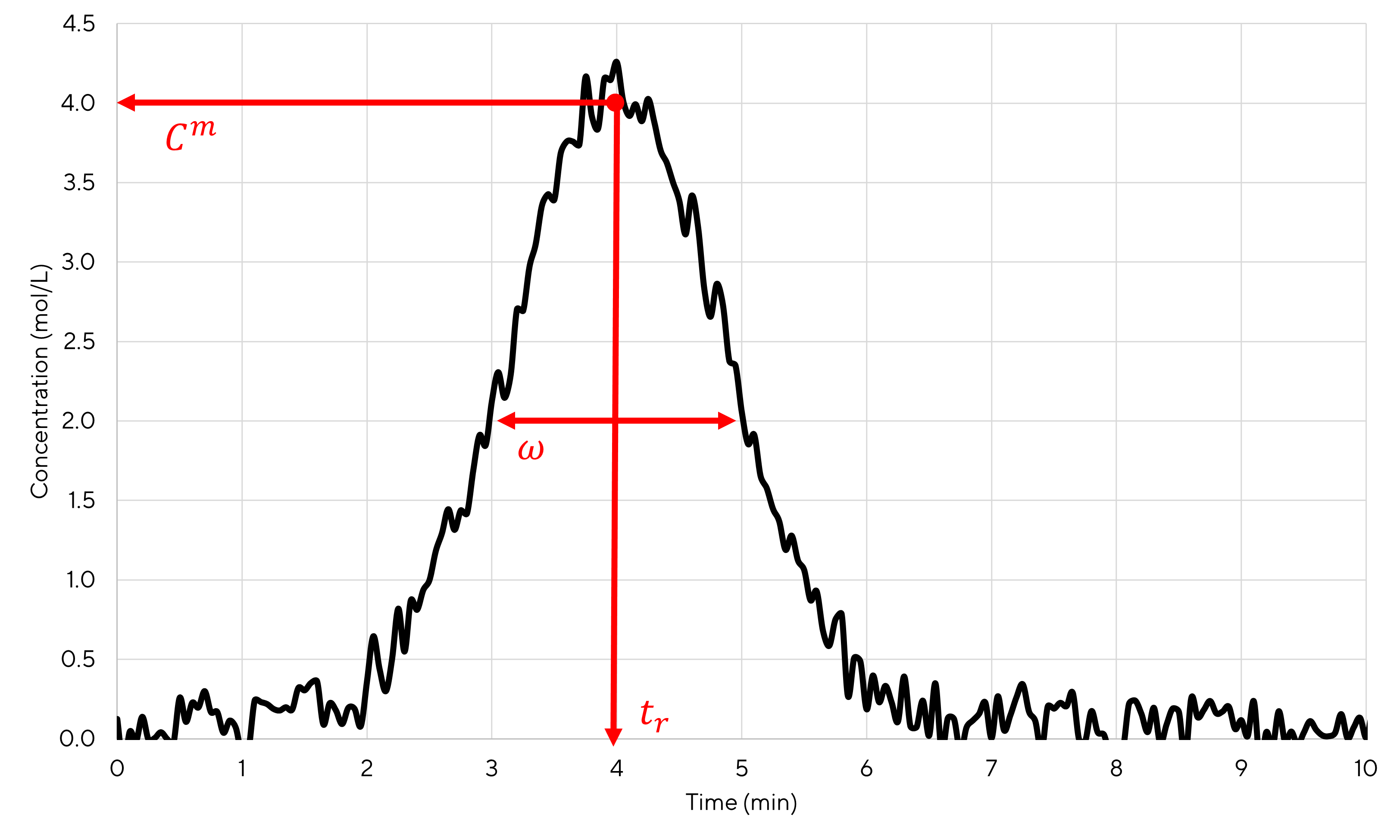
Figure 3.1: Noisy experimental peak
By reading the plot, one can see that \(t_r=4~min\), \(C^m=4~mol/L\) and \(\omega = 2~min\). From these values it is also possible to calculate the number of plates using equation (2.9). A value of 22.16 is obtained. Then, using equations (2.8) or (2.11), it is possible to calculate the theoretical gaussian curve that fits the best the experimental curve. The result is shown in figure 3.2.
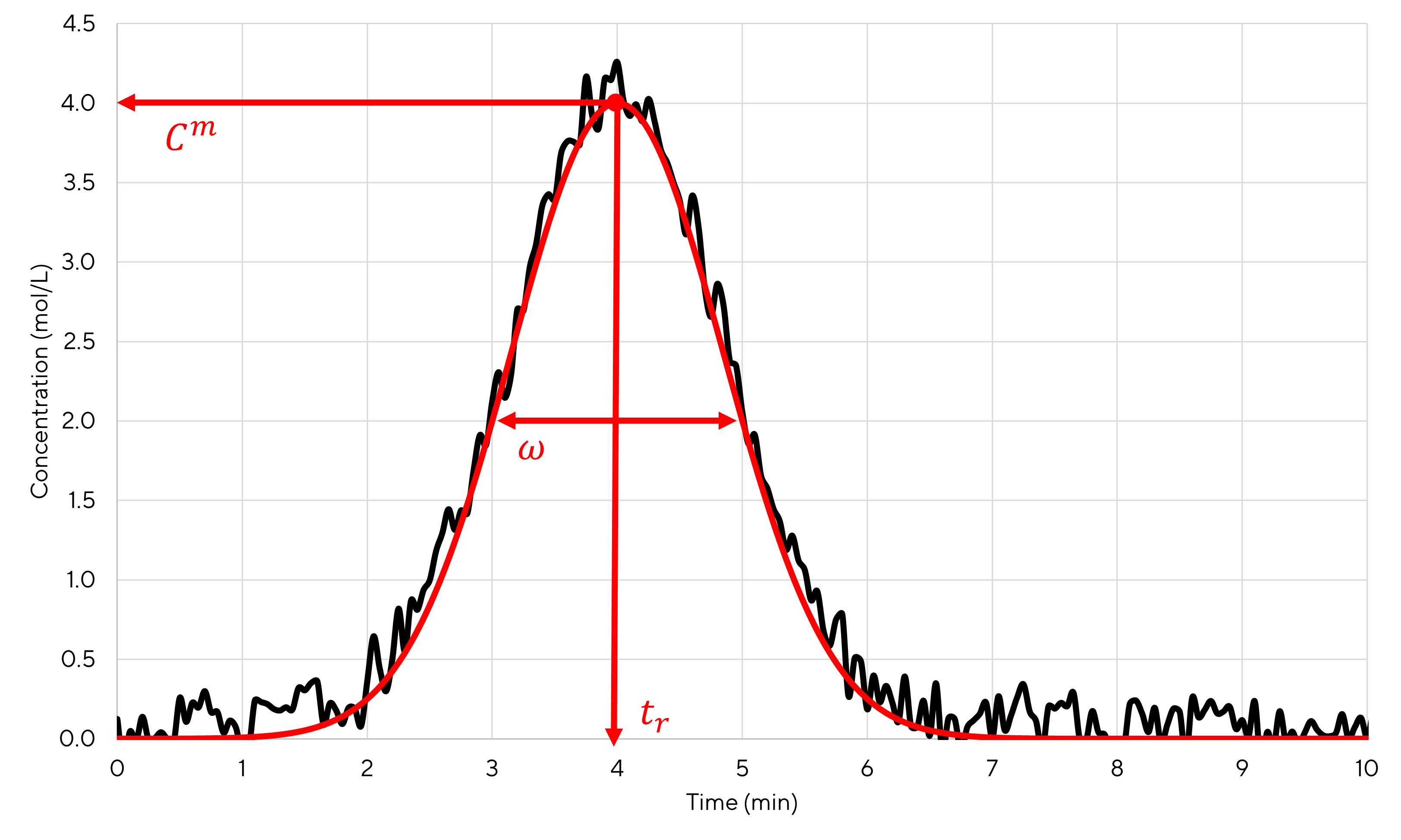
Figure 3.2: Simulated peak using a gaussian curve
3.2 Number of moles in a peak
In order to perform a mass balance, one must know what is the number of moles in the peak. First one must remember that \(n^{tot}=\int_{-\infty}^{+\infty}{C\left(t\right)}\times dV\) and therefore it is important to make volume \(V\) appear in the gaussian equation and not the time \(t\). Both terms are related by the flowrate \(Q\) according to the equation \(V=Q\times t\). Equation (2.8) then becomes:
\[\begin{equation} C\left(t\right) = C^m e^{-4\ln{2}\left(\frac{V/Q-t_r}{\omega}\right)^2} \tag{3.1} \end{equation}\]
The number of moles in the peak is then:
\[\begin{equation} n^{tot} = \int_{-\infty}^{+\infty}{C^m e^{-4\ln{2}\left(\frac{V/Q-t_r}{\omega}\right)^2}}dV = C^m \int_{-\infty}^{+\infty}{e^{-\left[\frac{2\sqrt{\ln{2}}}{Q\omega}\left(V-Qt_r\right)\right]^2}}dV \tag{3.2} \end{equation}\]
If one make the change of variable \(x = \frac{2\sqrt{\ln{2}}}{Q\omega}\left(V-Qt_r\right)\) then \(dV=\frac{Q\omega}{2\sqrt{\ln 2}}dx\) and
\[\begin{equation} n^{tot} = \frac{C^m Q \omega}{2\sqrt{\ln 2}} \int_{-\infty}^{+\infty}{e^{-x^2}}dx \tag{3.3} \end{equation}\]
The integral is known to be equal to \(\sqrt{\pi}\) (cf. this {post}) and finally:
\[\begin{equation} n^{tot} = C^m \times Q \omega \times \sqrt{\frac{\pi}{4\ln 2}} \tag{3.4} \end{equation}\]
Applying this equation to the peak depicted in figure 3.1 and assuming a flowrate of 1.5 mL/min, one finds that the total number of moles that leaved the column was:
\[\begin{equation} n^{tot} = 4\cdot 10^{-3} \times 1.5 \times 2 \times \sqrt{\frac{\pi}{4\ln 2}} = 0.0128~mol \tag{3.5} \end{equation}\]